Solve it fast.
Iterate without the heavy machinery.
A differentiable digital twin in closed form: one least-squares solve. No mesh, no time-stepping, no autodiff graph. Behind this text is steady Navier–Stokes past a classic 911, solved on fastlsq's closed-form basis and rebuilt by your browser from a few hundred kilobytes of coefficients.
A wind tunnel with
no mesh and no time-stepping.
The car is a showroom model, with panels, glass, chrome and an interior. The solver never meshes the air around it. It sees the car as one signed-distance function: a closed, lightly smoothed hull of the model. Collocation points are sampled in the air and projected onto that surface; the steady equations are linearised about the current guess, and each Newton step is one least-squares solve.
Divergence-free by construction
Velocity is a sum of plane waves t sin(W·x + b) with the polarisation
t ⟂ W. Each one has zero divergence, so ∇·u = 0 holds
exactly, at every point, and continuity never enters the solve.
Closed-form Stokeslets inside the body
Global sinusoids resolve a body's near-field slowly. Stokeslets and source doublets, seated just inside the surface, carry that structure: the method of fundamental solutions, as extra columns beside fastlsq's. Every column has analytic derivatives.
Redrawn from the coefficients
The page downloads the solved coefficients, rebuilds the velocity and pressure fields on your GPU, and integrates the streamlines from a smoke rake. No precomputed pictures, no flow data, just the closed form.
| equations | steady incompressible Navier–Stokes |
|---|---|
| Reynolds number | … |
| unknowns per solve | … |
| ∇·u | … |
| wall slip | … |
| momentum residual | … |
| Stokes flow past a sphere, vs exact | 5.8 × 10⁻⁷ rel. L² |
|---|---|
| Newton rows vs the full nonlinear residual | 5 × 10⁻¹¹ |
| normal equations vs QR, car drag | 1 × 10⁻⁵ rel. |
| stock-car drag, 9 600 vs 12 800 unknowns | 0.03% |
| stock-car drag, near-wall points ×2 vs ×3 | 1.2% |
| drag from the momentum flux through two boxes around the car, vs the surface | +3.3% · −1.2% |
Random sinusoids, one solve,
every derivative.
Drag N. Each feature is a frozen sinusoid sin(Wjx + bj);
only the coefficients β are solved for, by one least-squares call. Nothing here is
precomputed: the solve runs in your browser on every frame.
One β. Every derivative, exact.
β is solved once, against order 0. Every curve below is then read off the same coefficients. No re-fit, no finite differences, no autodiff graph. The analytic derivative (solid) lands on the true one (dashed) at every order.
A surrogate over a
random Fourier basis.
The basis
The unknown is expanded in a fixed basis of random sinusoids
φj(x) = sin(Wj·x + bj), with
Wj and bj drawn once and never updated.
Why it works
Averaging enough random Fourier features recovers the Gaussian RBF kernel (Bochner). Smooth solutions live in that RKHS, so a few hundred sinusoids span the space you need.
The fit
β comes from a single least-squares call. Because every feature is a plane
wave, differentiating just multiplies each coefficient by
Wjk and shifts the phase by
kπ/2.
One skeleton.
Many inverse problems.
An inverse problem needs a forward model you can differentiate, evaluated thousands of times. fastlsq gives you both: the operator assembles in closed form, the system factors once, and every subsequent solve is a back-substitution whose gradient rides back through the same factor.
Pick a problem. Only the operator line changes; the loop around it is identical every time.
| unknown | … |
|---|---|
| observations | … |
| forward model | … |
| what fastlsq gives | … |
…
…Compose any operator.
One formula handles it.
Every snippet on this page is executed against the released package before publishing. The numbers in the comments are real output.
import fastlsq as fl
from fastlsq.problems.linear import Helmholtz2D

result = fl.solve_linear(Helmholtz2D(), scale=5.0)

u = result["u_fn"]        # closed form, call it anywhere
m = result["metrics"]

m["val_err"]      # 2.3e-08
m["method_used"]  # 'svd'  (auto-selected)
m["rank_used"] # 261 of 1500 featuresrandom features: val_err varies run to run around 10⁻⁸
import torch
from fastlsq import Op
from fastlsq.basis import SinusoidalBasis

# Helmholtz:  Δu + k²u = f
L = Op.laplacian(d=2) + 10.0**2 * Op.identity(d=2)

basis = SinusoidalBasis.random(2, 1500, sigma=5.0)
x     = torch.rand(800, 2, dtype=torch.float64)

A = L.apply(basis, x)      # (800, 1500), closed form
g = basis.gradient(x)      # (800, 2, 1500), no autodiff
No graph is built. L.apply and basis.gradient
evaluate closed-form expressions, so cost is independent of derivative order
and nothing is retained for a backward pass.
Two problems, end to end.
Both are scripts in the repository. Every number below is their printed output.
Inverse heat-source localisation
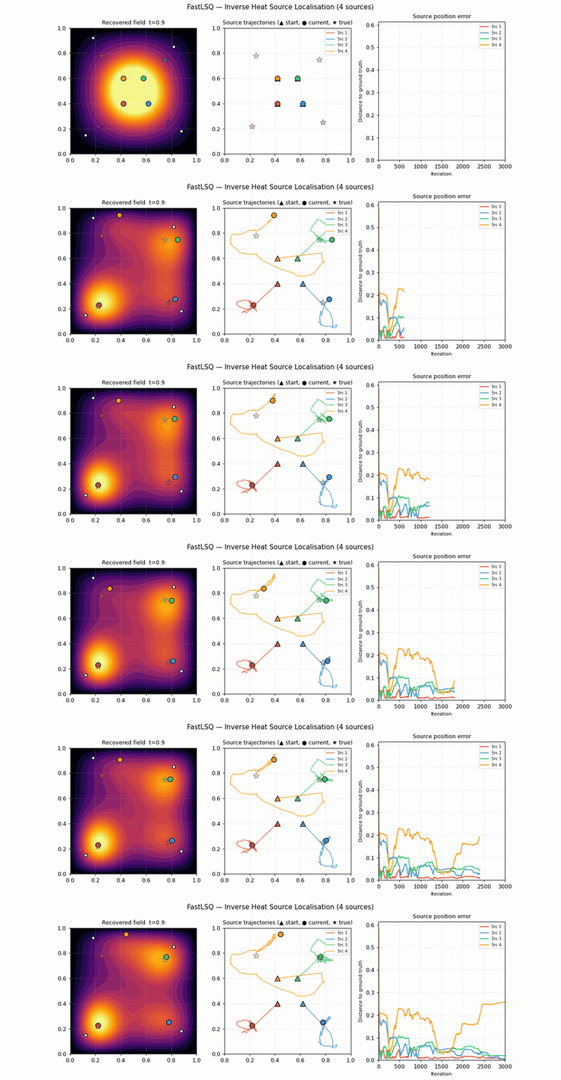
Four hidden heaters warm a plate. Four sensors record a temperature series as heat diffuses. From those 4 × 60 = 240 numbers, recover 24 unknown source parameters: position, shape and strength.
The forward model is the full space–time heat equation, and the search needs a complete PDE solve at every step. The (PDE + BC + IC) operator is assembled and Cholesky-factored once; each forward solve is then a back-substitution, and the gradient over all 24 parameters returns through the same factor.
| features | 2100 | observations | 240 |
|---|---|---|---|
| unknowns | 24 | iterations | 3000 (L-BFGS-B) |
| median |Δpos| | 0.013 | mean |Δpos| | 0.071 |
Three of four sources land within 0.02; the fourth does not. It settles 0.26 away with its intensity off by 130%, a local minimum of a genuinely non-convex problem. The mean above is dominated by that single miss, which is why the median is quoted beside it. Multi-start or continuation is the fix, and the point of a forward solve this cheap is that you can afford either.
examples/inverse_heat_source.py ↗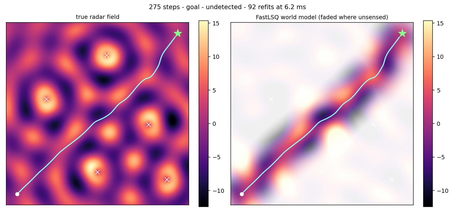
Stealth navigation: a twin refit in the loop
A drone crosses a radar interference field with no map: only a five-point cross of samples at its own position, streaming in as it moves. Every three steps it refits a surrogate over everything sensed so far (one Tikhonov least-squares solve), then steers on that surrogate's analytic gradient.
| features | 1000 | refits | 92 per episode |
|---|---|---|---|
| refit cost | 6.1 ms median | episode | 275 steps |
| peak exposure | 44.7 | detector at | 60.0 |
The ablation is the argument. Switch the gradient term off and drive straight at the goal: the detector trips at step 133 of what is otherwise a 275-step crossing. Steering on the closed-form gradient finishes 26% under the threshold. The twin is only trusted where the drone actually sensed, hence the fade in the right-hand panel.
examples/stealth_navigation.py ↗What changed in 0.7.1.
A correctness and hygiene release, 9 October 2026. The package was audited line by line; every defect below was reproduced on 0.7.0 before it was fixed, and each fix has its own regression test. The closed forms were re-verified against autograd and finite differences and are unchanged. 0.7.0, the week before, added the steady Navier–Stokes solver the wind tunnel above runs on.
load_checkpoint now reads with torch.load(weights_only=True),
so a crafted checkpoint can no longer execute code on load. State is stored as
tensors; a file written by 0.7.0 or earlier needs allow_pickle=True
and should only come from a source you trust.
Solves no longer reset the global random generator (repeated trials were
identical). set_device() is honoured by every module. The nonlinear
solver forwards your tolerances on the continuation path. A 1-D right-hand side
in solve_lstsq no longer gives a silent wrong-shaped result.
Learnable bandwidth: cached solves for vector outputs, dtype and device in
scalar mode, a ridge-consistent gradient, no hidden weight decay. Boundary
projection is scale-free; check_problem no longer false-alarms in
float32 and checks boundary data.
Newton reuses the accepted line-search Jacobian, one assembly fewer per
iteration with identical results. The import-time float64 default is documented
and can be switched off with FASTLSQ_KEEP_DEFAULT_DTYPE=1.
MirrorBasis accepts symbol and integral operators. The test suite is
order-independent and grew from 282 to 318 tests.
Full notes.
CHANGELOG.md explains
every fix and its cause ·
GitHub release ·
PyPI 0.7.1 ·
Zenodo 10.5281/zenodo.23267564.
Upgrade with pip install -U fastlsq.
The paper.
Method, proofs, ablations and the benchmark suite are in Sulc, A., FastLSQ: Solving PDEs in One Shot via Fourier Features with Exact Analytical Derivatives, arXiv:2602.10541.
@misc{sulc2026fastlsq,
  author        = {Sulc, Antonin},
  title         = {{FastLSQ}: Solving {PDEs} in One Shot via {Fourier}
                   Features with Exact Analytical Derivatives},
  year          = {2026},
  eprint        = {2602.10541},
  archivePrefix = {arXiv},
  primaryClass  = {math.NA},
  doi           = {10.48550/arXiv.2602.10541},
  url           = {https://arxiv.org/abs/2602.10541}
}